
But it may, if there is a good independent reason to think that X influences Y.
But it may, if there is a good independent reason to think that X influences Y.

\[Y = slope \times X + intercept\]
Simplest way two variables can be modeled as related to one another
\[Y_i = \beta_0 + \beta_1X_i + \epsilon_i\]

\[Y_i = \beta_0 + \beta_1X_i + \epsilon_i\]
Once you decide on a line, then the value of Y equals:


A residual represents the distance between the predicted value from the regression, and the actual value.
Another way to think about the residual: a single value from the normally distributed error term.
The squared residual is calculated as such:
\[d_i^2=(Y_i - \hat{Y}_i)^2\]
The best line minimizes the residual sum of squares
\[ RSS=\sum\limits_{i=1}^n(Y_i - \hat{Y}_i)^2\]
We could do a Monte Carlo approach: try a bunch of slopes passing through \((\bar{X},\bar{Y})\) and calculate the RSS, then pick the smallest, but math offers a simpler solution.
Recall the sum of squares: \[\ SS_Y = \sum\limits_{i=1}^n(Y_i - \bar{Y})^2\]
Sample variance: \[\ s^2_Y=\frac{\sum\limits_{i=1}^n(Y_i - \bar{Y})^2}{n-1}\]
SS equivalent to: \[\ SS_Y = \sum\limits_{i=1}^n(Y_i - \bar{Y})(Y_i - \bar{Y})\]
With 2 variables, we can define sum of cross products \[\ SS_{XY} = \sum\limits_{i=1}^n(X_i - \bar{X})(Y_i - \bar{Y})\]
By analogy to the sample variance, we define sample covariance \[\ s_{XY} = \frac{\sum\limits_{i=1}^n(X_i - \bar{X})(Y_i - \bar{Y})}{(n-1)}\]

From \(-\infty\) to \(\infty\)
\[\ s_{XY} = \frac{\sum\limits_{i=1}^n(X_i - \bar{X})(Y_i - \bar{Y})}{(n-1)}\]

From \(-\infty\) to \(\infty\)
\[\ s_{XY} = \frac{\sum\limits_{i=1}^n(X_i - \bar{X})(Y_i - \bar{Y})}{(n-1)}\]
By hand on whiteboard
x <- c(2 , 4, 3)
y <- c(1, 5, 6)
In ordinary least squares regression (OLS), the slope of the best fit line is defined as: \[ \frac{covariance\ of\ XY}{variance\ of\ X}\]
Or: \[\hat{\beta}_1 = \frac{s_{XY}}{s^2_X} = \frac{SS_{XY}}{SS_X}\] note: this simplifies because both are divided by same denomenator
The intercept is easy to find, because the best fit line passes through \((\bar{X},\bar{Y})\). Thus: \[ \bar{Y} = \hat{\beta}_0 + \hat{\beta}_1 \bar{X} \]
Or:
\[ \hat{\beta}_0 = \bar{Y} - \hat{\beta}_1 \bar{X}\]
Recall: \[Y_i = \beta_0 + \beta_1X_i + \epsilon_i\]
Regression assumes that that \(\epsilon\) is a random normal variable with mean 0 and variance of \(\sigma^2\), which is related to the scatter around the line.
We estimate \(\sigma^2\) like this: \[\frac{RSS}{n-2}\]
The square root of this is standard error of regression: \[\hat{\sigma}^2=\sqrt{\frac{RSS}{n-2}}\]
In a linear relationship, the total variance we want to explain is \(SS_Y\).
Some variance is attributable to our error term (measured by \(RSS\)).
The remaining variance is explained by our regression, thus: \[SS_{reg}=SS_Y-RSS\]
Therefore: \[SS_Y=SS_{reg}+RSS\]
This is referred to as partitioning a sum of squares.
This leads to calculation of \(r^2\), AKA the coefficient of determination
\[r^2 = \frac{SS_{reg}}{SS_Y}=\frac{SS_{reg}}{SS_{reg} + RSS}\]
The square root of this value is known as \(r\) or the product-moment correlation coefficient.
Note: the sign of \(r\) comes from the sign of the slope of the line.
You will always get parameter estimates for the intercept and slope. The next question is: are they signficant?
The slope measures the strength of the effect of \(X\) on \(Y\). The slope is a measure of effect size
| Source | Degrees of Freedom (df) | Sum of squares (SS) | Mean Square (MS) | F-ratio | P-value | |
|---|---|---|---|---|---|---|
| Regression | 1 | \(SS_{reg}=\sum\limits_{i=1}^n (\hat{Y}_i-\bar{Y})^2\) | \(\frac{SS_{reg}}{1}\) | \(\frac{SS_{reg}/1}{RSS/(n-2)}\) | F dist | |
| Residual | n-2 | \(RSS=\sum\limits_{i-1}^n(Y_i - \hat{Y}_i)^2\) | \(\frac{RSS}{(n-2)}\) |
We can also construct confidence intervals around our parameter estimates (formulae not shown).
Notice that our intervals are narrowest near the mean, and fatter the further you go away from mean.


myModel <- lm(response~predictor)
summary(myModel)
##
## Call:
## lm(formula = response ~ predictor)
##
## Residuals:
##    Min     1Q Median     3Q    Max
## -6.332 -1.288  0.029  1.307  6.137
##
## Coefficients:
##              Estimate Std. Error t value Pr(>|t|)
## (Intercept) -1.082286   0.623277  -1.736   0.0828 .
## predictor    0.311143   0.006218  50.036   <2e-16 ***
## ---
## Signif. codes:  0 '***' 0.001 '**' 0.01 '*' 0.05 '.' 0.1 ' ' 1
##
## Residual standard error: 1.96 on 998 degrees of freedom
## Multiple R-squared:  0.715,  Adjusted R-squared:  0.7147
## F-statistic:  2504 on 1 and 998 DF,  p-value: < 2.2e-16
plot(lm(response~predictor))

Any systematic correlation between the residuals and the fitted is bad.
Systematic departures from linearity can show up in the residual plots
response <- predictor^2 + rnorm(1000, sd=50)
plot(lm(response~predictor))

RMA regression assumes there is error in both X and Y
Minimizes an orthogonal residual sum of squares (along the major axis)
Show on white board
Model II regression requires a separate package lmodel2
In bioanthro literature, this regression is known as RMA (reduced major axis), but known in this package as MA (RMA in this package is something else)
The function is different, but the call is still simple.
library(lmodel2)
results <- lmodel2(response~predictor)
print(results)
##
## Model II regression
##
## Call: lmodel2(formula = response ~ predictor)
##
## n = 1000   r = 0.8318485   r-square = 0.691972
## Parametric P-values:   2-tailed = 1.943335e-257    1-tailed = 9.716673e-258
## Angle between the two OLS regression lines = 6.614198 degrees
##
## Regression results
##   Method  Intercept     Slope Angle (degrees) P-perm (1-tailed)
## 1    OLS  0.8163301 0.2927504        16.31741                NA
## 2     MA -0.2438352 0.3033804        16.87677                NA
## 3    SMA -5.0856439 0.3519276        19.38838                NA
##
## Confidence intervals
##   Method 2.5%-Intercept 97.5%-Intercept 2.5%-Slope 97.5%-Slope
## 1    OLS     -0.3997441        2.032404  0.2806177   0.3048831
## 2     MA     -1.5022970        1.005865  0.2908500   0.3159985
## 3    SMA     -6.3165411       -3.896451  0.3400039   0.3642694
##
## Eigenvalues: 108.3025 3.485197
##
## H statistic used for computing C.I. of MA: 0.0001325621
20 minutes

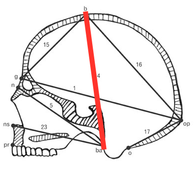
We are going to look at the scaling relationship between overall size and BBH (basion-bregma-height) in humans and fossil hominins
heads - Howell Craniometric Datafossils - Fossil DataCalculate the geomean for each individual in both data sets using the variables GOL, BBH, XCB, BNL, BPL, ASB
Add this data to a new column called geomean
geomean <- function(x, na.rm = TRUE) {
  product <- prod(x, na.rm = TRUE)
  n <- sum(!is.na(x))
  geo <- product ^ (1/n)
  return(geo)
  }
Do an Ordinary Least Squares regression of log(BBH) as a function of log(geomean) for the modern data and a separate one for the fossils
Make a plot of log(BBH) as a function of log(geomean)
How do the fossils compare to the modern humans?
How does LB1 (H. floresiensis) compare to other species?