Multivariate Statistics
Multivariate Data
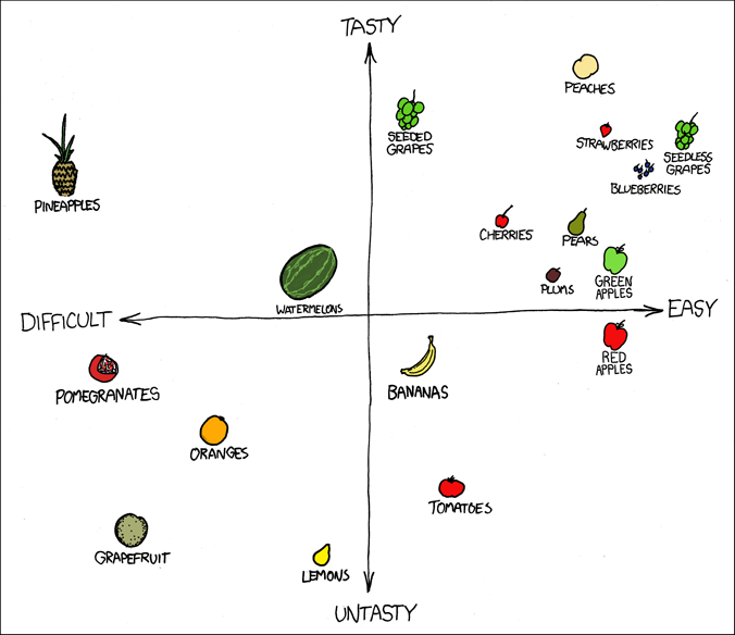
Often we collect many different variables
We want to answer questions like:
- how are the variables related?
- are their differences in the means and variances of the variables?
- can we look at a composite of some of these variables to simplify our data?
These questions are the domain of multivariate statistics
Covariance Matrices
Recall the sample covariance for two variables, calculated from the sum of cross-products
\[\ s_{XY} = \frac{\sum\limits_{i=1}^n(X_i - \bar{X})(Y_i - \bar{Y})}{(n-1)}\]
Covariance Matrices
With a multivariate sample comprising \(p\) variables, we can define a sample covariance matrix:
\[ S = \left[\begin{array}{ccc} s_{11} & s_{12} & .. & s_{1p}\\ s_{21}& s_{22} & .. & s_{2p} \\ .. & .. & .. & .. \\ s_{p1} & s_{p2} & .. & s_{pp} \end{array}\right]\]
What do the diagonal elements represent?
Covariance Matrices
var(iris[,-5])
##              Sepal.Length Sepal.Width Petal.Length Petal.Width
## Sepal.Length    0.6856935  -0.0424340    1.2743154   0.5162707
## Sepal.Width    -0.0424340   0.1899794   -0.3296564  -0.1216394
## Petal.Length    1.2743154  -0.3296564    3.1162779   1.2956094
## Petal.Width     0.5162707  -0.1216394    1.2956094   0.5810063
Correlation Matrices
Recall the correlation coeffiecient for two variables, which is a scaled version of the covariance.
\[ correlation\ coeffiecient = \frac{cov\ XY}{(sd\ X \times sd\ Y)}\]
or more formally:
\[ r = \frac{s_{xy}}{(s_{X} \times s_{Y})}\]
Correlation Matrices
We can then compute the correlation matrix for a multivariate sample of \(p\) variables.
\[ R = \left[\begin{array}{cccc} 1 & r_{12} & .. & r_{1p}\\ r_{21}& 1 & .. & r_{2p} \\ .. & .. & .. & .. \\ r_{p1} & r_{p2} & .. & 1 \end{array}\right]\]
Why are the diagonal elements all 1?
Correlation Matrices
cor(iris[,-5])
##              Sepal.Length Sepal.Width Petal.Length Petal.Width
## Sepal.Length    1.0000000  -0.1175698    0.8717538   0.8179411
## Sepal.Width    -0.1175698   1.0000000   -0.4284401  -0.3661259
## Petal.Length    0.8717538  -0.4284401    1.0000000   0.9628654
## Petal.Width     0.8179411  -0.3661259    0.9628654   1.0000000
Multivariate Distance Metrics
With a single variable (e.g. femur length) it is easy to conceptualize how far apart two observations are.
- Femur A = 25cm
- Femur B = 30cm
- How far apart are these individuals in terms of femoral length?
As we add more measurements, it becomes less obvious to tell how “far apart” two specimens are.
If the Humerus of indivual A is 15cm and the Humerus of indiviaual B is 22cm, then how far apart are individuals A and B?
We need a multivariate distance metric.
Euclidian Distance
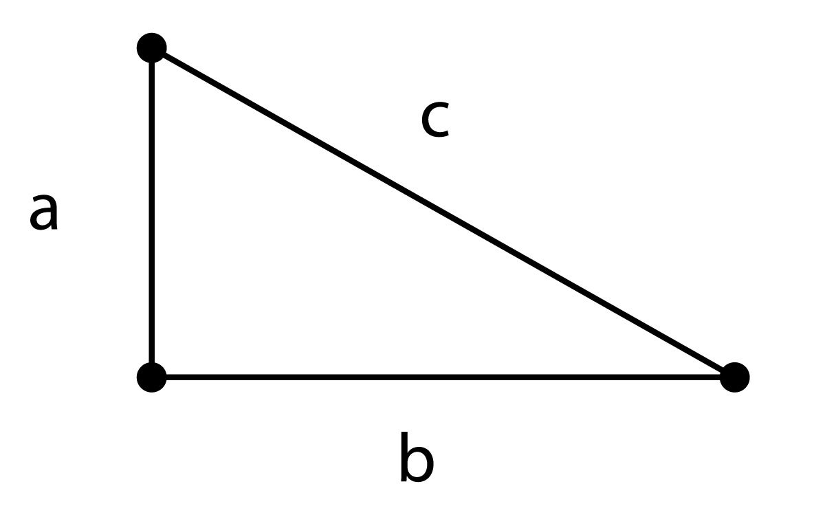
\[c = \sqrt{a^2 + b^2 }\]
Euclidian Distance
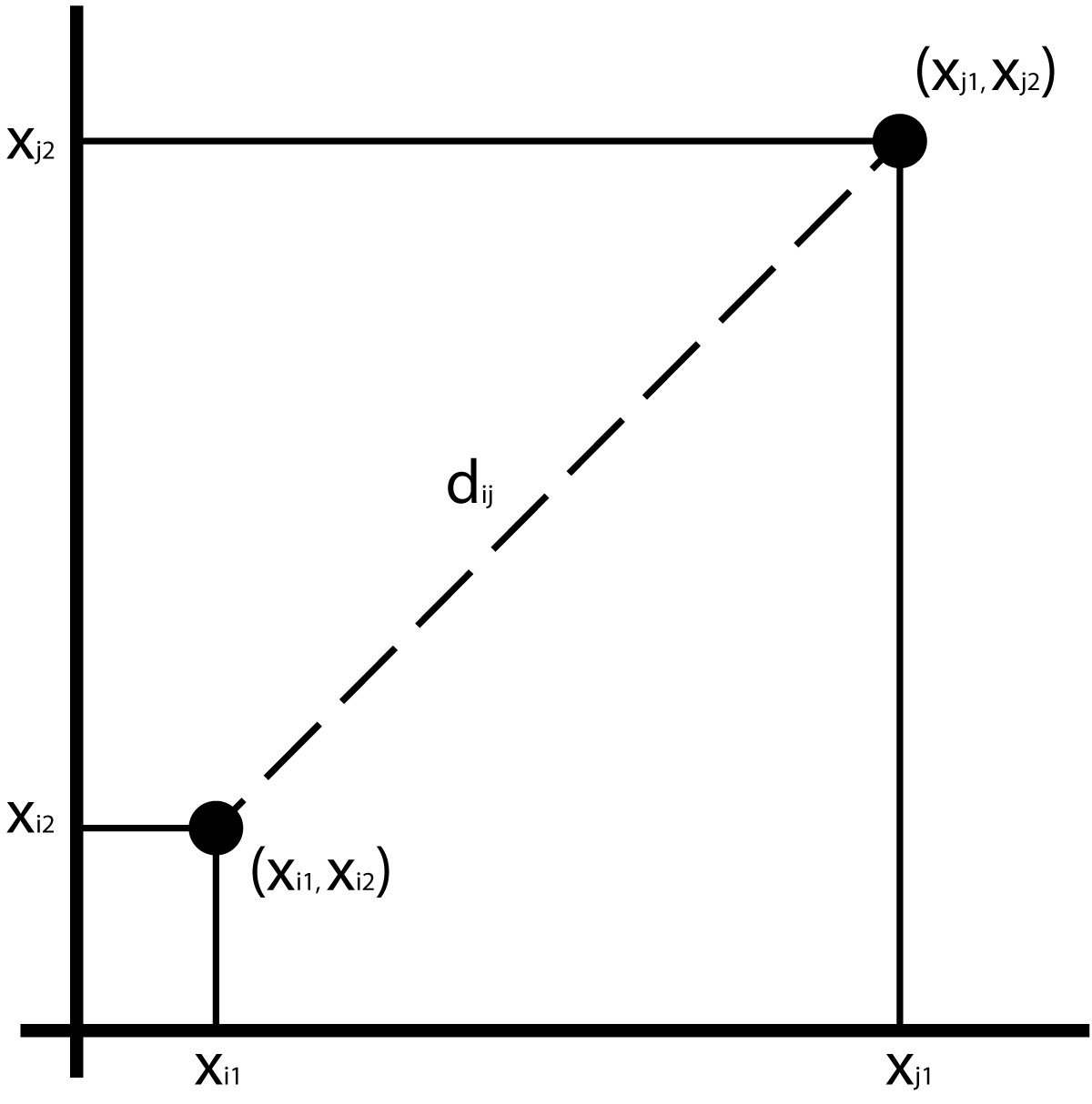
Assuming 2 variables, we can compute the distance as the hypotenuse of a triangle:
\[d_{ij} =\sqrt{(x_{i1} - x_{j1})^2 + (x_{i2} - x_{j2})^2}\]
Euclidian Distance
We can compute a Euclidian distance for any number of variables:
\[d_{ij} = \sum\limits_{k=1}^p \sqrt{ (x_{ik})^2 - (x_{jk})^2 }\]
Euclidian Distance
Euclidian distances can easily be swamped by large scale measurements.
To avoid this, you can calculate a z score by subtracting the mean of the measurement and dividing by the standard deviation.
The dist() function in R calculates Euclidian distances by default.
Mahalanobis Distance
Calculates the distance of an observation from its multivariate centroid (mean of all measurements), taking into account the covariance of the variables.
\[D^2_{ij} = \sum\limits_{r=1}^p \sum\limits_{s=1}^p (x_{r} - \mu_{r})\ v^{rs} (x_{s} - \mu_{s})\]
where \(v^{rs}\) is the covariance between variables \(r\) and \(s\)
Mahalanobis Distance from centroid (triangle)

Mahalanobis Distance
means <- c(mean(iris$Sepal.Length), mean(iris$Sepal.Width), mean(iris$Petal.Length), mean(iris$Petal.Width))
VCV <- var(iris[,-5])
mhdists <- mahalanobis(iris[,-5], means, VCV)
mhdists[1:10]
##  [1] 2.134468 2.849119 2.081339 2.452382 2.462155 3.883418 2.862108 1.833300
##  [9] 3.384073 2.375218
Distance Matrices
Several multivariate techiques derive directly from matrices of distances.
Calculate a Euclidian Distance Matrix
dist(iris[1:5,-5])
##           1         2         3         4
## 2 0.5385165
## 3 0.5099020 0.3000000
## 4 0.6480741 0.3316625 0.2449490
## 5 0.1414214 0.6082763 0.5099020 0.6480741
Cluster Analysis
start with a distance matrix
assume each individual is in a group of 1
join individuals within a given distance into a group
continue joining groups until there is a single group
visualize with a tree (dendrogram)
Cluster Analysis
library(dplyr) #load dplyr just to have the pipe %>%
iris[,-5] %>% dist %>% hclust %>% plot

Principal Components Analysis
Goal is to “summarize” variation in multivariate data
Reducing dimensionality of dataset is called ordination and many multivariate techniques fall in to this category
Reduce the number of dimensions needed to describe most of the variance
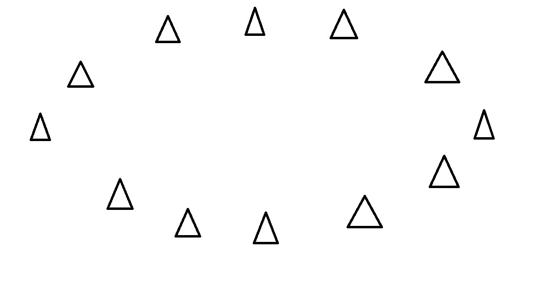
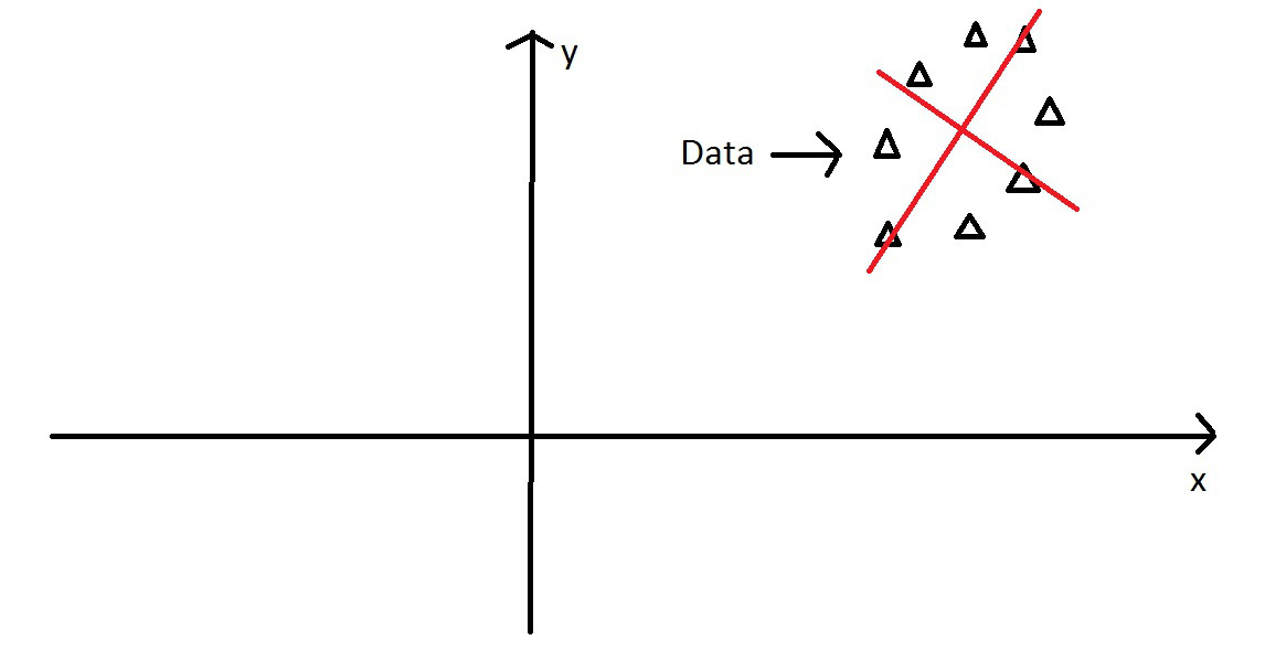
PCA - Intuitively
Start with some data points
PCA - Intuitively
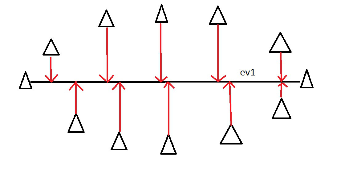
Examine the variance of the points along some axis…
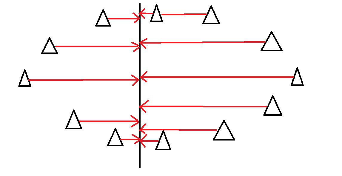
PCA - Intuitively
This axis covers much more variance in our points…
PCA - Intuitively
Imagine these points in some XY coordinate system….
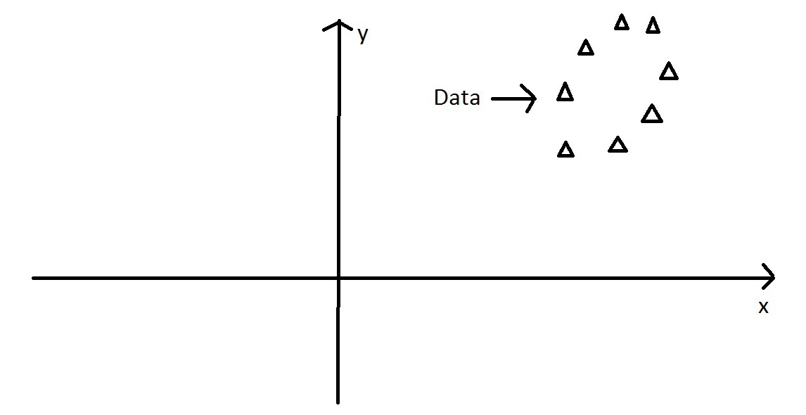
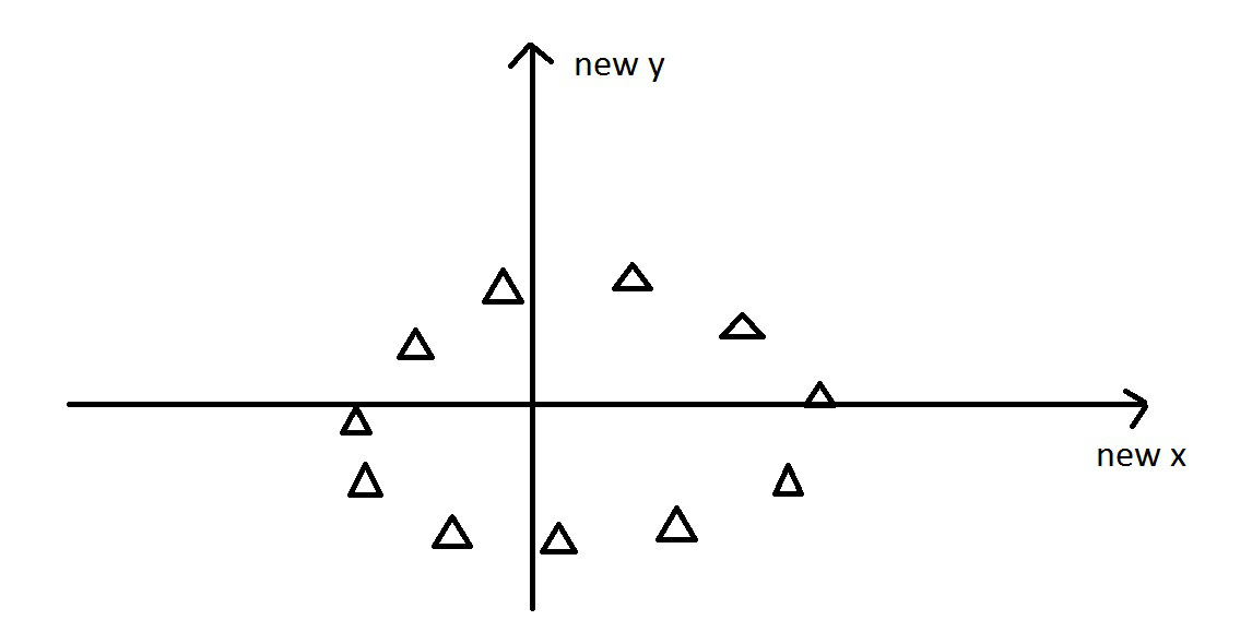
PCA - Intuitively
We can still find the axis of maximum variation….
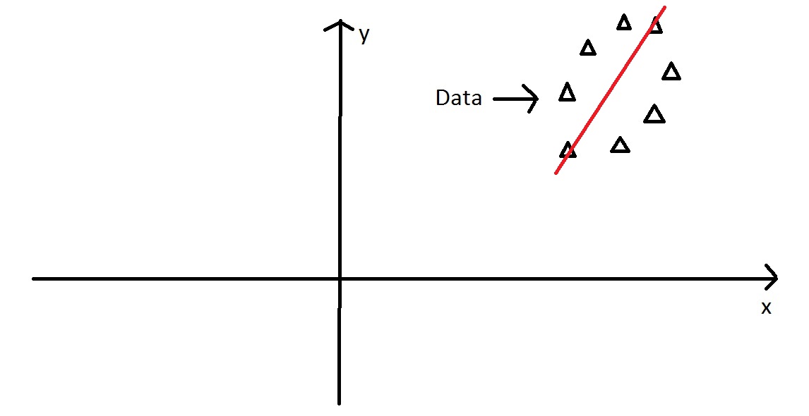
PCA - Intuitively
Then we find the orthogonal axis, 90\(^\circ\) from major axis
PCA - Intuitively
Next, we rotate the data to use the two new principal components axes we found…
Eigenvalues and Eigenvectors
Consider a system of linear equations:
\[a_{11}x_1 + a_{12}x_2 + ... + a_{1n}x_n = \lambda x_1 \\ a_{21}x_1 + a_{22}x_2 + ... + a_{2n}x_n = \lambda x_2\\ ... \\ a_{n1}x_1 + a_{n2}x_2 + ... + a_{nn}x_n = \lambda x_n\]
Eigenvalues and Eigenvectors
These equations only hold true for some values of \(\lambda\), which are called the eigenvalues.
There are up to \(n\) eigenvalues.
These equations can be solved for a given eigenvalue (e.g., the \(ith\)), and the resulting set of values is called the \(ith\) eigenvector.
I don’t expect this to be crystal clear if you haven’t studied linear algebra!
PCA - operationally
- Starting with the covariance matrix
- The eigenvalues of this matrix are the variances explained by each PC
- The eigenvectors of this matrix are the contributions of each original variable to the PC
- The eigenvectors can be thought of as “transformation equations” to convert a datapoint from the original space to the PC space
PCA - more details
- We start with \(p\) variables for \(n\) individuals
- The first PC is the linear combination of all the variables:
- \(PC1 = a_1X_1 + a_2X_2 + ... + a_pX_p\)
- PC1 is chosen to vary as much as possible for all the individuals, subject to the condition that the sum of the squared \(a\) terms is 1
- Subsequent PCs are uncorrelated with the prior PCs
PCA - even more details
- (sometimes) scale and center your variables to have a mean of 0 and variance of 1.
- Calculate the covariance matrix (this will be a correlation matrix if you did step 1)
- Find the eigenvalues (variances of the PCs) and corresponding eigenvectors (the loadings for each variable) for the covariance/correlation matrix
- Ignore the components that (hopefully) explain very little variance, and focus on the first few components
Principal Components Analysis in R
There are 2 functions in R
prcomp()princomp()
These differ in their implementation and default arguments, but provide similar results.
However, prcomp() is preferred for numerical accuracy
PCA - Example
These are bivariate plots of the familiar iris dataset, with 4 numerical variables. Lets do a PCA to summarize all the variation in a smaller number of variables.

PCA - Example cont.
There are two main ways to call the PCA function:
- provide a dataframe with ONLY numeric columns, in which case the PCA is run on all the columns, or
- use a one sided formula (just like when you specify ggplot2 facetting formulae) to specify which variables to put into the PCA.
I like the second option, because it is more explicit exactly which variables are going in.
irisPCA <- prcomp(iris[,1:4],
                  scale=TRUE, center=TRUE)

#note both of these are equivalent

irisPCA <- prcomp(~Sepal.Length + Petal.Length + Petal.Width + Sepal.Width,
                  data=iris,
                  scale=TRUE, center=TRUE)
PCA - Example cont.
Now that we have a PCA object, we can look at the output:
irisPCA
## Standard deviations (1, .., p=4):
## [1] 1.7083611 0.9560494 0.3830886 0.1439265
##
## Rotation (n x k) = (4 x 4):
##                     PC1        PC2        PC3        PC4
## Sepal.Length  0.5210659 0.37741762 -0.7195664  0.2612863
## Petal.Length  0.5804131 0.02449161  0.1421264 -0.8014492
## Petal.Width   0.5648565 0.06694199  0.6342727  0.5235971
## Sepal.Width  -0.2693474 0.92329566  0.2443818 -0.1235096
summary(irisPCA)
## Importance of components:
##                           PC1    PC2     PC3     PC4
## Standard deviation     1.7084 0.9560 0.38309 0.14393
## Proportion of Variance 0.7296 0.2285 0.03669 0.00518
## Cumulative Proportion  0.7296 0.9581 0.99482 1.00000
PCA - Example cont.
To plot irisPCA you can use the base biplot(irisPCA) function which is ugly but effective, but using the ggfortify package is much easier.
library(ggfortify)
autoplot(irisPCA, data=iris, colour="Species", loadings=TRUE, loadings.label=TRUE)
 ## PCA - Example cont.
Notice on the previous example that we are color coding by Species, which is a column that exists in the original iris dataset, but DOES NOT exist in the PCA model object (because PCA only works on numeric columns). This is why you have to use data=iris, colour="Species" to get the color coding right. Also ggfortify isn’t as forgiving as ggplot2 is on how you spell ‘colour’.
PCA - Example cont.
I prefer to plot my own PCA plots using ggplot2.
If you look inside the irisPCA object using the str() function you will see that there are a bunch of components. You are most interested in the one called x because this contains the new coordinates for each observation in the new PCA space.
head(irisPCA$x)
##         PC1        PC2         PC3          PC4
## 1 -2.257141  0.4784238 -0.12727962  0.024087508
## 2 -2.074013 -0.6718827 -0.23382552  0.102662845
## 3 -2.356335 -0.3407664  0.04405390  0.028282305
## 4 -2.291707 -0.5953999  0.09098530 -0.065735340
## 5 -2.381863  0.6446757  0.01568565 -0.035802870
## 6 -2.068701  1.4842053  0.02687825  0.006586116
PCA - Example cont.
Now we can make a new dataframe for our plot, using the x values from the PCA, and the Species column from the original data
forPlot <- data.frame(irisPCA$x, Species=iris$Species)
ggplot(data = forPlot, mapping=aes(x=PC1, y=PC2, color=Species)) + geom_point()

PCA - Example cont.
Note…it is harder to plot the eigenvectors (the arrows) if you are doing it yourself. I never use them because I don’t find them that helpful. If you do, I suggest going with ggfortify